RAW format and noise

Introduction

This short article summarizes my attempt at a better understanding of some image sensor characteristics that have increasingly become a part of digital camera vocabulary and my-medium-is-better-than-your-medium controversies. It is not the intent of this article to explain how CCD/CMOS image capturing devices work, but rather highlight some of their characteristics and their limitations using a simple experiment. In order to do that, as every TIFF or JPEG output has already been heavily post-processed, raw data is analyzed.

RAW format, CRW in particular

A "raw" format of a digital camera stores data from a sensor array in its original unmodified, unsharpened, and un-interpolated form. This is not to say that it is really the data measured by the sensor, as some post-processing may be already done in hardware, but it is as close as one can get to the measured data, and it is also the starting point for any software that turns the data into an image.

There is a number of steps involved in converting the RAW data into an image. In no particular order, the data must be color-interpolated since most digital sensors employ color masks thereby measuring at each pixel only some of the color and light intensity information. Based on the characteristics of the color mask and the spectral sensitivity of the sensor, some mapping between the measured numbers and actual colors must be used and results must be converted into one of the commonly used color spaces, with the appropriate gamma. White balance is applied in part to emulate our own visual perception, in part to even out the spectral response of individual channels of the sensor. The image is usually sharpened to compensate the effect of the anti-aliasing filter in front of the sensor. This special blurring filter is used to suppress color interpolation artifacts such moire, sampling and interpolation artifacts such as jagged lines etc. A noise reduction of some sort may be applied. Some of these steps may overlap. All in all, converting a RAW file is not a trivial task and involves a decent amount of well documented steps and also some inexact science to make the image look good to us. This is why good RAW processing software is often not given away for free.

Canon RAW format (CRW) is like other RAW formats proprietary and Canon offers a development library that will convert RAW files. Unlike the Nikon's NEFF, CRW in Canon's SLRs has used compression since inception and its first appearance. Nikon now uses a compressed NEFF format too in the D2h, and to make things more interesting, the new Eos 1D II is supposed to feature a new compression. The first Canon RAW format has been successfully decoded by Dave Coffin, a smart programmer from Boston, after months of attempts. Some of his code is used in many commercial software packages that now offer imports of RAW formats. Aside from headers, EXIF information and the optional JPEG, CRW stores the lowest two bits uncompressed since no compression works well for noise dominated data, and a lossless compression is used for the other ten. What noise, you ask - read on.

Noise

Noise is not some bad engineer's excuse for failing to design a perfect device. In fact, a good part of it is due to the quantum nature of the universe and cannot be avoided by any kind of image capturing medium. This part is called the shot noise and is proportional to the square root of the signal. Then there is a number of other sources of noise that engineers attempt to reduce - read-out circuitry noise (for example reset noise, output amplifier noise), noise associated with the image capturing element itself such as dark current noise (mostly the result of imperfections in the semiconductor) or just plain non-uniformity of individual photosites on the sensor. Kodak claims that, for example, dark current noise varies by a factor two from lot to lot, which makes every camera quite unique. Kodak has a lot of information about noise, ways of dealing with it, ways of increasing sensor sensitivity on their web site. It makes for an intriguing reading material. More on that possibly some other time, let us now see how well Canon engineers and manufacturing have done in the case of Canon 10D.

Experiment setup

The camera (Canon EOS 10D) with a 70-200 lens zoomed out to 200 has been pointed at a matte white sheet of paper. The sheet was illuminated by diffused light from a north-facing window with partially closed beige blinds on a sunny day. The distance from the window and the angles involved ensured that the sheet of paper was evenly illuminated. In order to avoid picking up any texture in the paper, the camera was placed as close as possible from the sheet, about 5 feet, the lens was focused at infinity and left wide open at f/2.8. The temperature in the room was a relatively high 74 degrees Fahrenheit.

A series of shots in a half stop increments was taken (starting from the camera metered value 1/60s down to 1/4000s and then up to 2s; the blinds were dimmed for the higher ISO). The shots were taken in quite short intervals and there is a remote possibility this has increased the noise somewhat. The results were evaluated on a 32x32 patch of pixels from the center of the frame (including 512 green pixel, 256 red and 256 blue pixels). To verify even illumination, the quality of results was checked by evaluating rectangular patches of 64x8 and 8x64 with virtually identical results. This experiment is, however, limited by the accuracy of the camera's shutter as well as a well documented noise dependence on the exposure time.

A source code of the program dcraw.c by Dave Coffin was modified to capture red, green, and blue pixel values from a Canon RAW file. The results were evaluated statistically by computing averages, minima, maxima, and standard deviations over the center patch for each of the color channels separately. The only preprocessing step that has been applied to the data is setting the black point by subtracting the reading of a masked part of the sensor from all the data.

Results

The measurements were carried out at two extreme ISO settings of the camera - 100 and 1600. In the figures, ISO 100 appears on the left and ISO1600 on the right. Exposure corresponding to 0 on the x-axis is given by the meter reading.

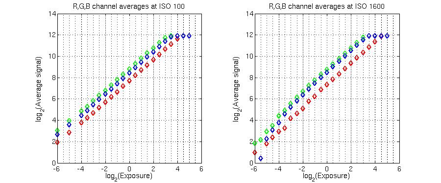
Figure 1 shows the averages over the center patch for each of the color channels as a function of exposure. There is a few properties to note here:

Each of the channels exhibits a linear response over much of the range of values until saturation is reached. This linear response is typical of CCD/CMOS light capturing devices. The range, measured from the red channel values in which the longest usable range was captured, is at least 10 EV (stops) at ISO 100. It may well be slightly more as the measurement below -6 are missing, though no more than 12EV, which is the A/D convertor range. However, the pixel to pixel resolution in the low part of the range will be compromised by noise. See below.
The green and blue channels have a higher sensitivity than the red channel. This is combined effect caused by the color of the illumination used and also a common characteristics of many CCD/CMOS devices given by their native spectral sensitivity. Since in post-processing, in this case, the output of the red channel then needs to be boosted when the white balance is applied, higher noise levels in the red channel result.

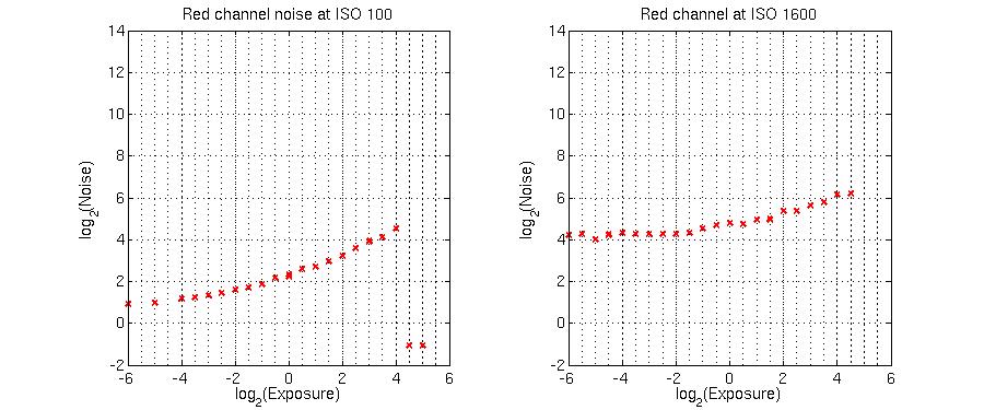
Figure 2 depicts noise measured as the standard deviation from the average value in the red channel (the other channels exhibit similar behavior) as a function of the exposure. The graph has three distinct subregions. On the left, the noise levels out as the noise floor is approached. In the center, the noise becomes shot noise dominated until the sensor saturation is reached, at which point the noise disappears but so does the usable signal response (cf. Figure 1).

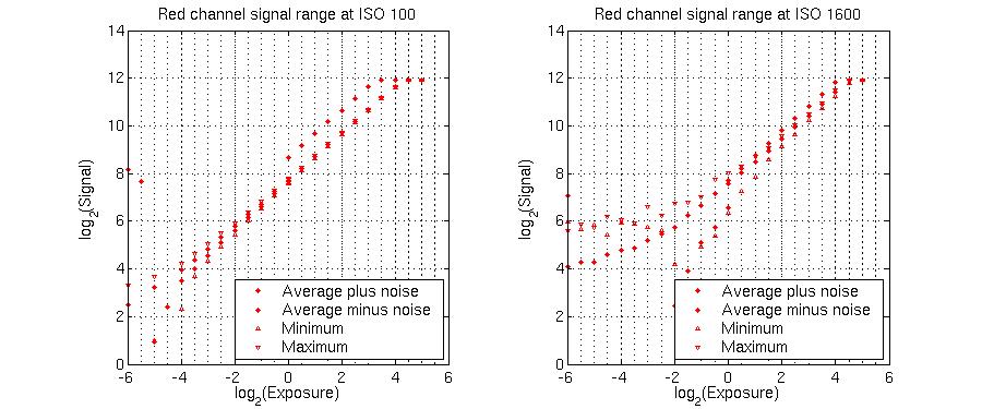
The next figure shows a composite of the previous two - the range of values in the red channel signal, given by taking the average signal and adding and subtracting the noise measured by the standard deviation, and also by the signal maxima and minima.

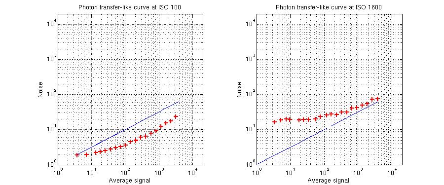
Figure 4 shows a variation of the so-called photon-transfer curve for the red channel - the x-axis shows the signal and the y-axis the noise. The dynamic range is often defined as the ratio of the noise floor, in this case about 2, and the full-well charge (maximum signal before saturation), which turns out to be about 3875, implying the range of 66dB. Also, the middle part of the graphs has a slope of about 1/2 (indicated by the blue line) confirming that the signal there is shot noise dominated as pattern noise non-uniformity would result in a linear increase in noise. Kudos to Canon for the on-pixel noise reduction. In fact, it would appear they have reduced the noise below the theoretical minimum. It is not so. The noise is measured by the standard deviation, which may not be entirely representative for the type of noise encountered, and most importantly, the noise and signal values in the graph are not on the same scale as the photon shot noise mentioned above, which may shift the graph left or right.

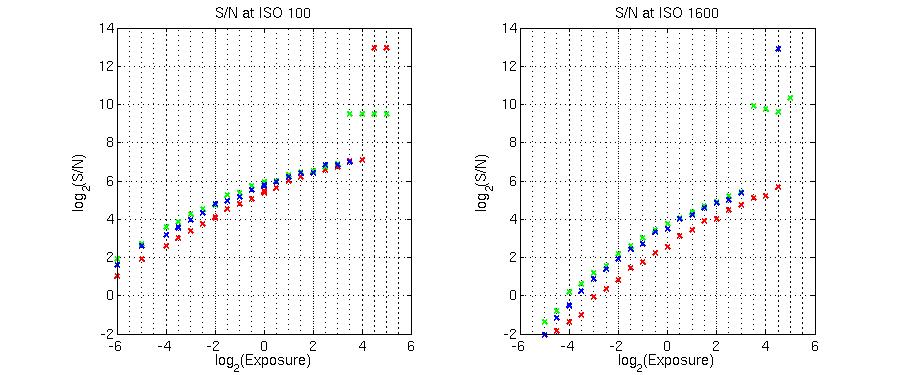
Finally, the S/N (signal to noise) ratio as a function of the exposure is displayed in Figure 5. If the useful range is defined by the range where the signal is not completely lost in the noise (and thus preserves small detail), the S/N ratio must be greater than one. The upper bound of the useful range is obviously the saturation point. Then, the useful range in the red channel is 9EV at ISO 100 and 7EV at ISO 1600. If all the channels are considered at the same time, these numbers are diminished, for the particular color of the light used, to 8EV and 5.5EV respectively.

Lessons learned

EOS 10d captures enough of a range of brightness in the photographed scene so one seldom needs to worry about it. Extremely contrasty situations which would be problematic with film will remain problematic. This, at least in some static situations, can be circumvented by shooting the same scene twice with different exposure settings. By their digital nature, the resulting images are straightforward to merge. The noise levels are very low helping to preserve low contrast and shadow detail. It is also important to realize that even in the noise dominated range of exposures, the average CCD/CMOS signal remains linear (cf. Figure 1 and Figure 5) so with some loss of resolution, some detail in the image can still be recovered. In other words, if the noise is objectionable, it can be smoothed out by noise reduction at the expense of resolution.

Even though software white balance can even out the disparity in spectral responses of individual color channels, it is still not time to toss away color compensating filters, especially if the best dynamic range is to be captured in situations with highly colored light. In this respect, it is highly desirable that a camera provide histogram information for each channel separately. In order to achieve the best S/N ratios, one should overexpose but make sure the sensor saturation (resulting in blown-out areas in the image) is not reached. This is tough to do in practice so bracketing may still be a good idea even on top of inspecting the histogram. The histogram separately for each channel will prove to be useful here also. However, from experience, the histogram alone may not reveal the damage done to the visual effect of the image by blown-out areas. This is reserved for inspecting the image at its final display size and thus the need for bracketing.

Let us finish by making a few comments about advantages of the RAW format as opposed to an in-camera JPG. In a lot of respects, the RAW format is an equivalent of a film negative and the post-processed JPG can be likened to a machine photographic print. If the machine settings are appropriate, the print is going to be reasonably close to what is achievable. On the other hand, if we happen to be printing a high contrast scene on a contrasty paper, fail to appply correct color masking, and even get the density wrong, the result may look horrendous. But we can go back to the negative and at least try and reprint to our liking. This is what the RAW format allows us to do. If the white balance, contrast, sharpness, compression have not been set correctly in camera, we can always modify them in the RAW conversion without magnifying artifacts introduced by the previous conversion. On top of that, the additional bit depth information can give us more latitude when it comes to tonality editing, e.g. to bring out shadows or prevent posterization.

Last updated: February 19, 2004
Please send any comments to

or, if you prefer, sign an entry in the guest book.